|
BIOMCON Infoletter 2013/#2 |
Bio-Math-Consulting |
|
|
|
|
|
|
|
||

|
Population Evolution Charts? What’s that? By Dr. Joachim Moecks, BIOMCON GmbH, Mannheim, Germany March 2013 |
|
|
Many clinical studies feature time-to-event endpoints (e.g. time to progression, time to relapse etc, usually studied with Kaplan-Meier displays). Now let us think of this common setting from another angle: We start with a full patient cohort at baseline and the events select patients out of this cohort. After some study time we have e.g. 60% of the patients left and so on (that’s what the Kaplan-Meier actually tells us). Now consider some covariate e.g. a histological tumor subtype – we now look at the selection by events with focus on this tumor subtype. To fix ideas, suppose that the study is in oncology (endpoint progression-free- survival) and at baseline the histological type of the tumor is analyzed (e.g. adeno or non-adeno).
Suppose at baseline there are 50 % adeno and 50% non-adeno tumors. What if after some study time (say, we have now 60% of the initial cohort) the percentage of adenocarcinomas increased to 70% in this group of 60% of the original patient cohort?
This tells us that the events selected predominantly non-adeno tumors – and thus the treatment seems to work better in adeno-tumors.
Population Evolution Charts (PEC) for these data are simple. The PEC here is simply the monitoring the percentage of adeno-tumors in the patient population over treatment time.
This is only an example. Depending on the medical context, we may replace in the example adenocarcinoma by any other interesting criterion e.g. sex, age in 2 groups (young vs old), or by a special diagnose group (histology, NYHA class) or by any other criteria. The nice thing with PECs is that they come as graphics, need no difficult (mathematical) assumptions and are easy to understand.
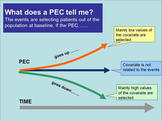
The basic principle of interpretation is illustrated in the graphic below. For the adeno example above (say adenocarcinoma receive the flag 1, while others are coded by 0), then we would see an increasing PEC over time – starting at 50% going up to 70% at later study times. Thus giving a clear indication, that whatever happened after study start – it does favour adenocarcinoma.
In what can a PEC help you? (illustrated in the graphics below)
|
|
|
|
In which data is the analysis by PECs useful? Whenever the study is big enough that you would consider Kaplan-Meier curves then PECs can be a useful tool. |
|
|
|
The usual analysis of covariates way would consider Cox proportional hazard model for obtaining hazard ratios. This model relies on a crucial mathematical assumption and PECs can be useful also to this end:
Real data examples illustrate these points:
The first example (graph 1) features the decline of percentage of males during the study. Clearly females benefit more from this treatment. We may accept that this is a steady decrease (despite of small random bumps). Therefore Cox-regression to find the hazard ratio between male and females could be a next step.
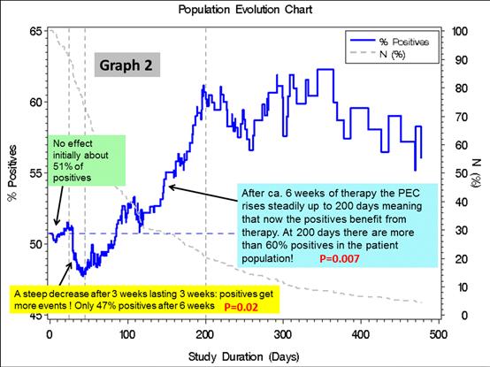
The second example (graph 2) shows a more complicated pattern. The PEC here features the percentage of biomarker positives over time. After a steep significant decrease – i.e. positives had more events than negatives – after 6 weeks the PEC rises steadily – i.e. now biomarker positives were better off !
Could this mean that in untreated patients, positivity indicates a bad prognosis – and after a latency the targeted treatment is able to reverse the situation and can deliver a clear benefit for biomarker positives?
The time dynamic shown by the PEC can thus help to develop interesting hypotheses. By the way, the application of overall Cox regression in graph 2 is strongly discouraged, since assumptions are grossly violated and the results would not be useful.
|
|
|

|
bioMcon GmbH | Max-Joseph-Str. 9 | D-68167 Mannheim | Tel. +49 (0) 621/1287361 | Email:info@biomcon.com |